Prelab/Background

At a high level, a Bayes filter operates on a prior belief. The prior belief is the robot's belief of its position based on sensors and control inputs. As new measurements are taken, and new control inputs are performed, that belief is updated to reflect the new information.

The pseuodo code for the Bayes filter is shown below. The Bayes filter uses a motion model and a sensor model to update the belief of the car's position. The motion model is used to predict the car's position based on the car's previous position and the control input (line 3). The sensor model is used to update the belief of the car's position based on the sensor measurements (line 4).

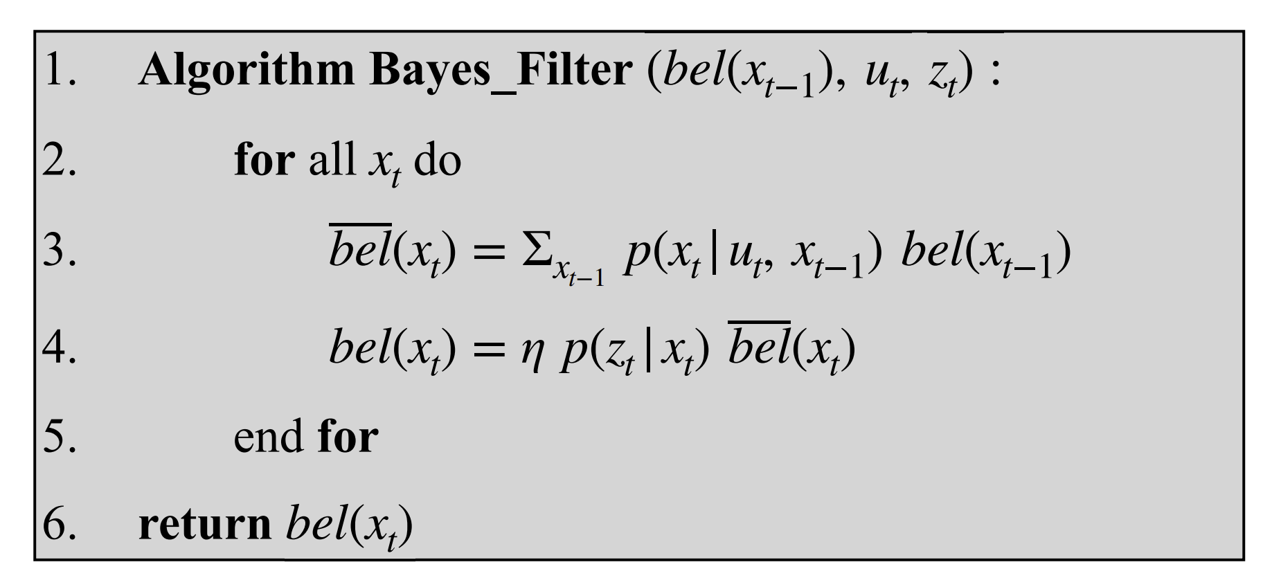
The filter is computed by iterating through all possible locations of the robot within its environment. To make this computable, the possible poses are discretized. Since the robot's state is 3-dimensional, the state space is a 3D grid, where each cell in the grid has an x, y, and theta position that corresponds to the x, y, and rotation of the robot.

Implementation

compute_control

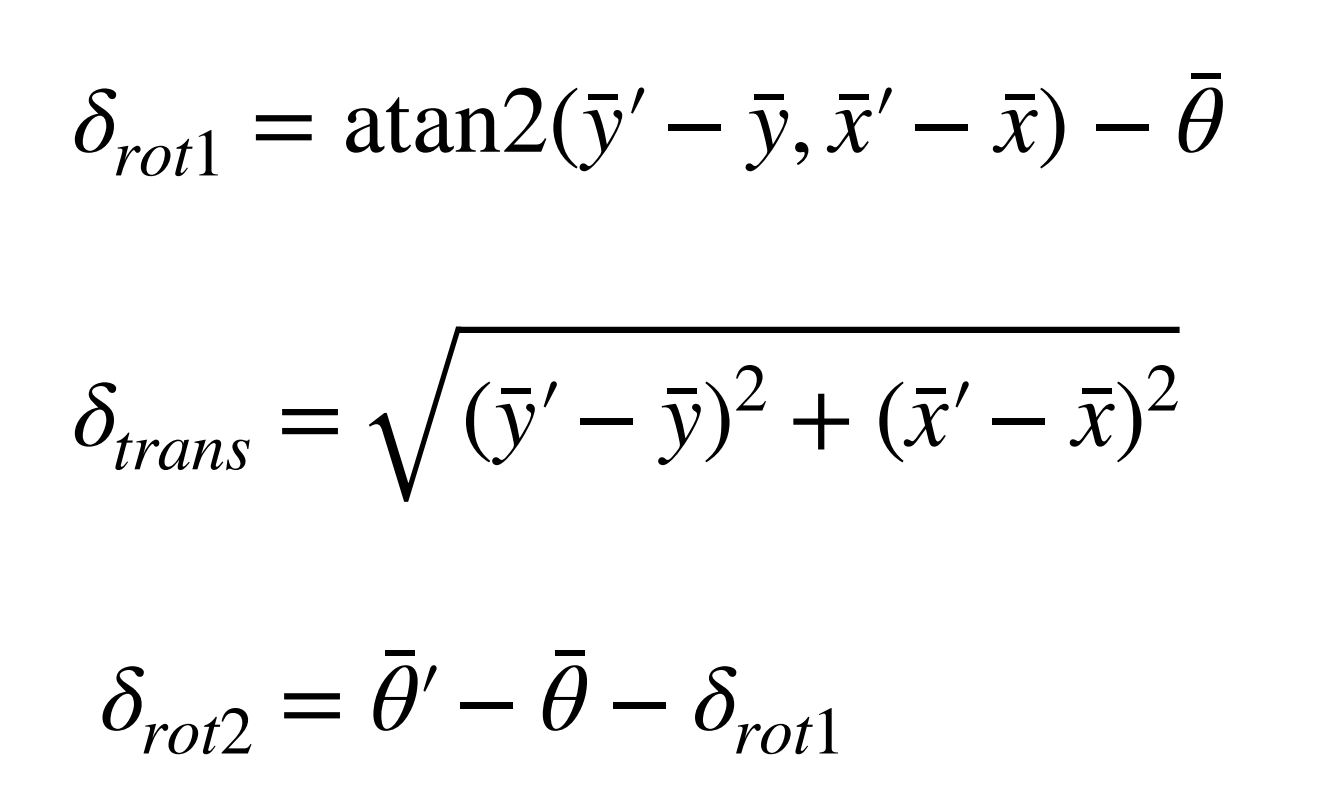
The prediction step of the Bayes filter relies on the motion model to compute the expected control input given a previous pose and a current pose. The control input is expressed as a rotation, a translation and a second rotation. The input poses are expressed as x, y, coordinates and theta for a degree of rotation.

The compute_control implementation is shown below. The function follows the derived odometry model parameters shown in ECE 4160 Lecture 18. Notably, math.degrees() function converts the angles to radians. The mapper.normalize_angle() call normalizes the input angle to the range [-180, 180).

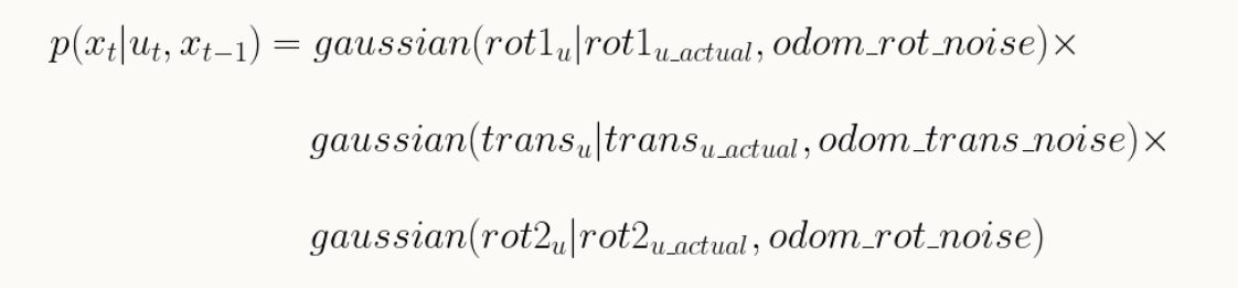
odom_motion_model

The motion model should calculate the probability that the robot reaches a position x' given the previous position x and the control input u. To calculate this, we first need to calculate the expected control input expected_u given the current and previous pose with the compute_control function. With a Gaussian distribution centered around the expected control input with a standard deivation of our degree of confidence in the odometry model, we can pass in each of the actual control parameters to the Gaussian distribution to get the probability of the robot reaching the position x' given the previous position x and the control input u. The odom_motion_model implementation is shown below.

prediction_step

With the motion model implemented, we can now implement the prediction step of the Bayes filter. The prediction_step function uses the previous belief loc.bel[cx,cy,ca] (the confidence that the car was in the location cx, cy, ca), and the motion model to calculate the probability the car is located in each position within the grid. This effectively implements line 3 of the Bayes Filter pseudocode shown above.

As mentioned in the lab handout, previous beliefs that are below 0.0001 do not need to be calculated. These beliefs contribute very little to the overall belief and can be ignored. The prediction_step function is shown below.

sensor_model

After the prediction step, a sensor model is used to update the belief of the car's position. The sensor model is based on an array of true observations for each position within the grid. The robot's sensor measurements are passed into a Gaussian distribution centered around the true measurement with a standard deviation that reflects the noise level of the sensor. Effectively, this calculates the probability of the robot's sensor measurements are similar to the true mesaurements for a position within the environment.

The sensor_model function is shown below.

update_step

The update step of the Bayes filter uses the sensor model to update the belief of the car's position. The update_step function takes in the previous belief and the sensor model to calculate the new belief. This effectively implements line 4 of the Bayes Filter pseudocode shown above.

Results

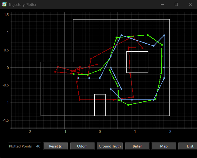
We can deploy our Bayes filter to the simulated environment to localize the robot. In the following plot, the ground truth (the actual position of the robot) is shown in green, the Bayes filter localization is shown in blue, and localization with the odometry model is shown in red. As shown in the plot, the Bayes filter localization is comparable to the ground truth, while the odometry model localization is not.

The logs below show the prediction and update step outputs of the Bayes filter. The logs include the ground truth pose, and the most probable state after each iteration of the prediction and update step, along with the probability. The Bayes filter works especially well when the robot is closer to a boundary and drives with a minimal rotations in its control input. This could be due to more accurate distance sensor readings when the robot is closer to walls.