LAB 9: Mapping
Orientation Control
The car's orientation is obtained using the IMU with DMP. See the DMP setup and angle wrapping implementation in the Lab 6 writeup.
The PD controller implemented in lab 6 is reused to control the car's orientation. The code is ommited in this writeup as the full code is included in lab 6. To allow for the car to turn at small angles, the proportional error term is increased. This allows the motor to reach a duty cycle high enough to overcome the static friction of the wheels when the error is small. After each step of the PD controller, the TOF sensor is read if data is ready. The TOF distance data, along with the car's orientation, and motor input are recorded.
Data is logged with calls to the following function. The distance and distance2 variables refer to outputs from the two TOF sensors. Only distance is used in post processing.
The following code snippet illustrates how the car is stepped through 36 angles from 0 to 360 degrees. The time.sleep(0.5) call ensures TOF sensor measurements are taken at each setpoint.
After the car finishes its 360 degree turn, a seperate command SEND_YAW_MAPPING_DATA is sent to the car to begin the transfer process of the recorded YawMappingDataBuffer data. 360 degree turns were executed at each of the required marked positions in the lab (-3,-2), (5,3), (0,3), (5,-3), along with (0,0) as an extra position.
The video below shows the car performing reasonable on-axis 360 degree turn.
The graphs below illustrate the motor input, the car's yaw, and the TOF sensor data over time.
-1-motor_input_and_yaw_vs_time.png)
-1-yaw_and_distance_vs_time.png)
Post Processing
Loading in data
Data is loaded to and loaded from a csv file. A load_data(..) function is defined that takes in arguments to indicate which dataset to load. After the load_data(..) function is called, the data is able to be manipulated in global lists. The load_data(..) implementation is shown below.
Polar Coordinates
As an initial sanity check that the recorded data is accurate, polar coordiante plots are created for the data recorded at each position. The polar coordiante plots are created with the following function. After converting the yaw to radians, each angle is mapped to a radius that corresponds to the distance recorded at that angle. The polar coordiante plot is then created using the matplotlib library. The polar coordiante plots are shown below.
-2-yaw_vs_distance_polar.png)
-2-yaw_vs_distance_polar.png)
-2-yaw_vs_distance_polar.png)
-2-yaw_vs_distance_polar.png)
-1-yaw_vs_distance_polar.png)
To confirm that the polar coordiante plots are correct across multiple trials, two plots are shown next to eachother. The result for the (0, 0) position is shown below.
-1-yaw_vs_distance_polar.png)
Converting to the global frame
To convert the global frame, we can use the transformation matrix below.
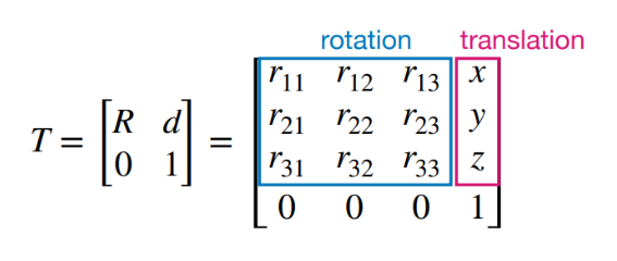
By orienting the car at the same initial position, the rotation matrix can be set to the identity matrix. The translation matrix is the x, y, and z-offsets of the car. Since we are not concerned with the z-axis, the transformation matrix is a 3x3 matrix instead.
The transform_data function processes sensor data (yaw and distance) collected from a robot at a given origin to generate global Cartesian coordinates for plotting. It first loads the data for a specified trial and origin. The angles are converted to radians and used to compute local Cartesian coordinates, where the X and Y components are derived as x = -distance * cos(yaw) and y = -distance * sin(yaw) for my specific mounting of the TOF sensor onto the robot. The robot's origin is converted from feet to millimeters, and a homogeneous transformation matrix is applied to translate the local points into the global frame. The full implementation is shown below.
Line 6 is an angle offset to account for some skew in the angle measurements. This is due to some drift by the DMP when the IMU is first initialized.
Line 8 is to account for a translational offset between the TOF sensor and the center of the car. This way, measurements are with respect to the center of the car.
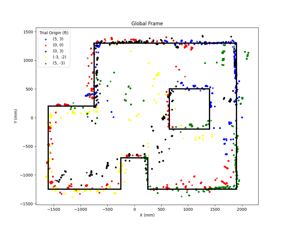
The global frames of each mapped position is shown below.
-global_frame.png)
-global_frame.png)
-global_frame.png)
-global_frame.png)
After overlaying the global frames over eachother, the following graph is obatined. If I were to redo this lab, I would take less TOF measurements or adjust TOF sensor parameters such as increasing timing budget or integration time to produce a cleaner and less noisy graph.
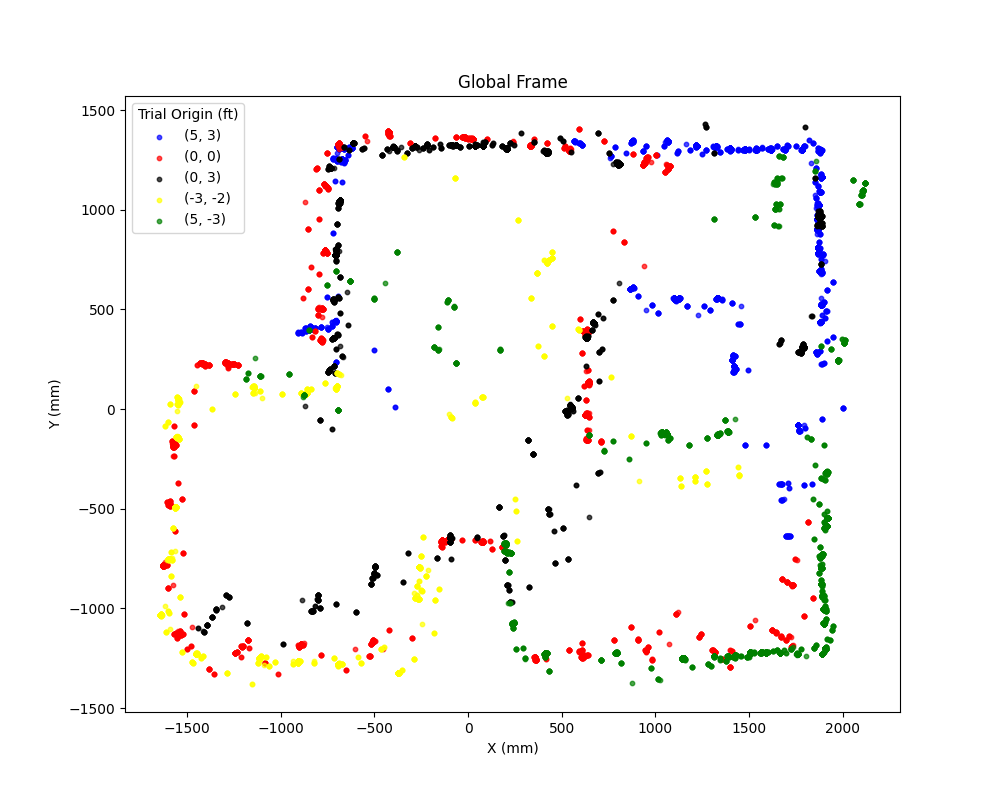
With a global map, we can overlay this map with lines that represent the walls of the obstacles. The walls are represented as a list of tuples as shown below. The lines are then added to the combined global map to yield the following graph.