LAB 2: IMU
Set up the IMU
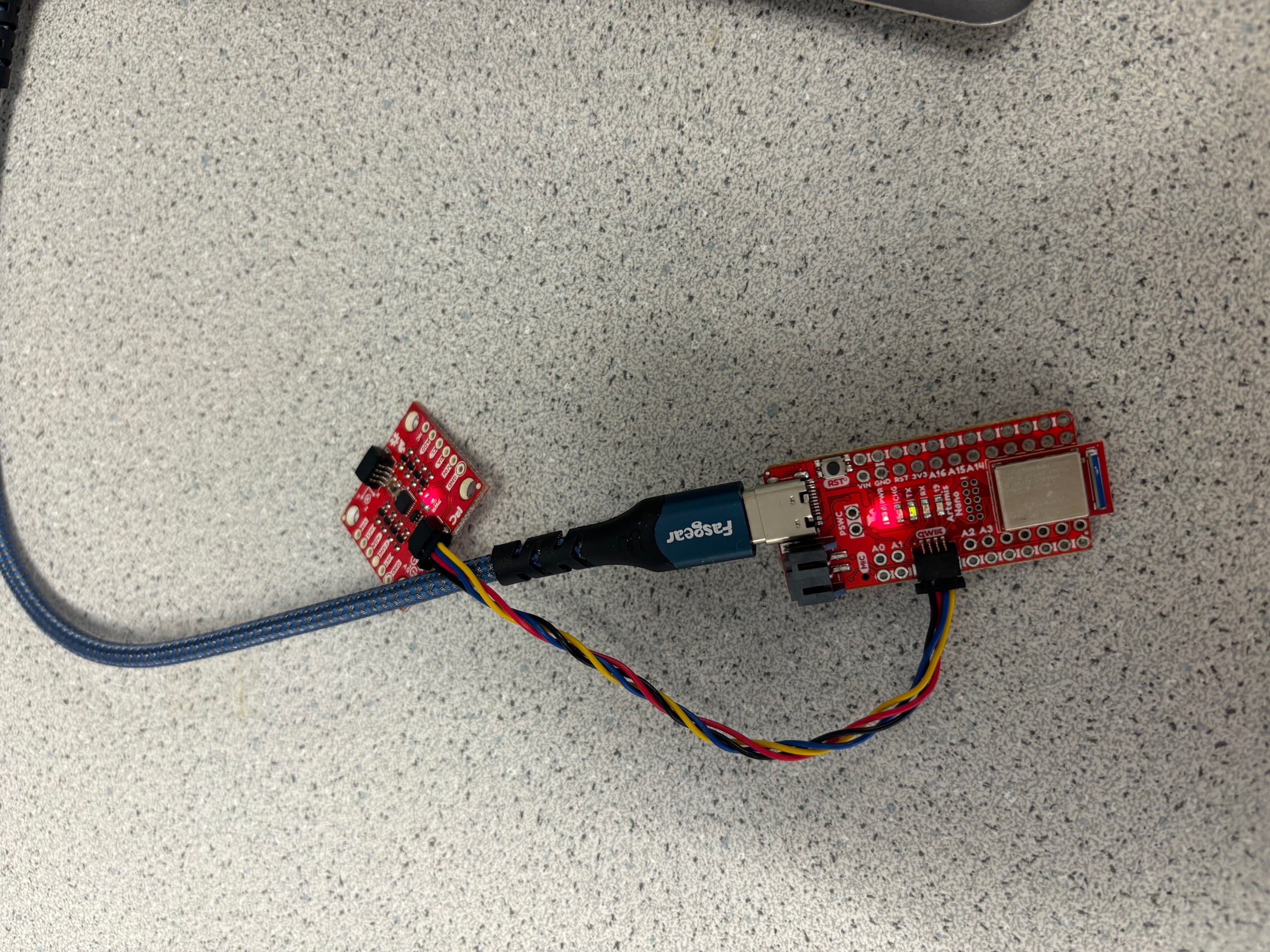
The IMU is connected to the Artemis Nano via a QWIIC connector.
The following video demonstrates the Example1_Basics.ino script form the ICM 20948 Arduino Library.
The AD0_VAL value represents the last bit of the I2C address. According to the script, the SparkFun 9DoF IMU breakout defaults to 1, and the value becomes 0 when the ADR jumper is closed. This flexibility in the I2C address allows us to have multiple devices on a single I2C bus.
The acceleration data shows the magnitude of acceleration in milli G's. Accelerometer outputs are split into the X, Y, and Z directions. When the accelerometer is placed on a flat surface, the magnitude of the acceleration in the Z direction is ~1G, corresponding to Earth's gravity. The gyroscope data showed the current angular velocity in the X, Y, and Z axis in degrees per second.
Accelerometer
The pitch and roll values are calculated from the accelerometer data. The pitch value is the angle between the X-axis and the horizontal plane, while the roll value is the angle between the Y-axis and the horizontal plane. The pitch and roll values are calculated using the following functions:
The atan2_custom(..) function returns a value between -pi and pi the pitch and roll
in radians. The
ACCEL_[PITCH/ROLL]_CONVERSION and ACCEL_[PITCH/ROLL]_OFFSET have
values of 1 and 0 respectively. These will be calibrated using two-point calibration in a later
section.
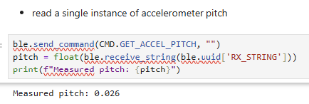
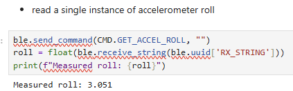
Bluetooth commands GET_ACCEL_PITCH and GET_ACCEL_ROLL are also
implemented. The uncalibrated pitch and roll at -90, 0, and 90 degrees is shown using the
bluetooth interface.
| Degrees | Pitch (radians) | Roll (radians) |
|---|---|---|
| -90 | 0.026 | 3.051 |
| 0 | 1.529 | 1.576 |
| 90 | 3.043 | 0.008 |
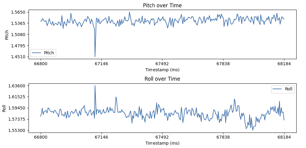
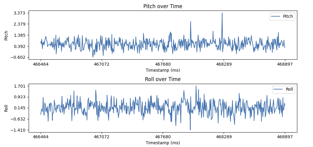
The following graph shows the calculated pitch and roll values before calibration for an IMU flush to a flat surface. The accelerometer pitch and roll has a +/- 0.015 radians of noise. Furthermore, the pitch and roll should be 0, but is off by a factor of ~1.53 and ~1.58 radians respectively. Notably, the accelerometer has little drift. Data was recorded around 66 seconds after the Artemis was flashed, and the pitch and roll are still similar to what was measured at 0 degrees in the table above.
The accelerometer's scaling accuracy can be improved by calibrating the pitch and roll values. The accelerometer's pitch and roll values are calibrated using a two-point calibration method. The calibration points are set to -90 and 90 degrees. The calibration values are calculated using the following code:
The p_90_accel_[pitch/roll] and n_90_accel_[pitch/roll] variables are
the uncalibrated
values of pitch and roll when the IMU is held at 90 and -90 degrees respectively. Since the
desired angles range from
-90 to 90, the desired range is 180. The deisred range is divided by the actual range to find
the conversion factor.
The accel_[pitch/roll[_offset_raw variables houses the uncalibrated pitch and roll
values when the IMU is held with 0 pitch and 0 roll. The accel_[pitch/roll]_offset
variable is calculated by multiplying the raw offset with our previously calculated conversion
factor.
A bluetooth command CALIBRATE_ACCEL is implemented to calibrate the pitch and roll
by sending our calculated conversion factors and offsets to the Artemis board. The conversion
factors will then be used when the Artemis calculates pitch and roll values, meaning subsequent
GET_ACCEL_[PITCH/ROLL] commands will give us readings with the correct scale.
| Degrees | Pitch (radians) | Roll (radians) |
|---|---|---|
| -90 | -91.474 | -91.749 |
| 0 | 0.757 | -0.335 |
| 90 | 95.746 | 89.713 |
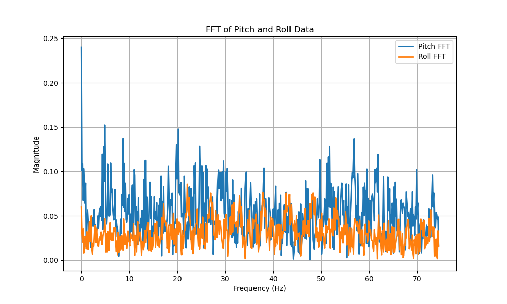
Before implementing a low-pass filter, the noise needs to be characterized to find an appropriate cut-off frequency. The noise was characterized with an FFT for cases where the IMU was still and faced a disturbance. The FFT was calculated by sending labeled Pitch and Roll data with timestamps to calculate the frequency between data points. Numpy's fft library was then used to fit the time-domain data to the frequency domain.
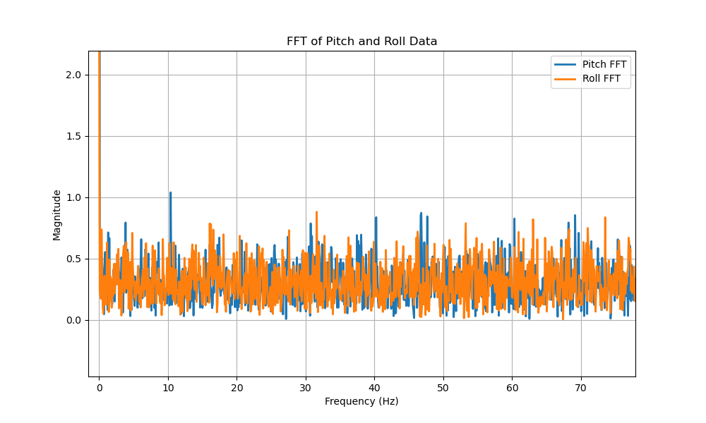
Based on the FFT, we see most noise occurs at frequencies greater than 5 Hz. Thus, we can set our cut-off frequency to be 5 Hz. Using the following equations, we can find our \(\alpha\) value for our low-pass filter.
\( dt = \frac{1}{\text{Sample Rate}} = \frac{1}{196 \text{ Hz}} = 0.005102 \text{ seconds} \)
\( RC = \frac{1}{2 \cdot \pi \cdot f_{\text{low-pass}}} = \frac{1}{2 \cdot \pi \cdot 5 \text{ Hz}} = 0.032 \text{ seconds} \)
\( \alpha = \frac{dt}{dt + RC} = \frac{0.005102}{0.0.005102 + 0.032} = 0.138259 \)
We can now use \( \alpha \) to calculate the low-pass filter value for the pitch and roll using the following equation from lecture 3.
\[ \theta_{\text{LPF}}[n] = \alpha \cdot \theta_{\text{RAW}} + (1 - \alpha) \cdot \theta_{\text{LPF}}[n-1] \]
\[ \theta_{\text{LPF}}[n-1] = \theta_{\text{LPF}}[n] \]
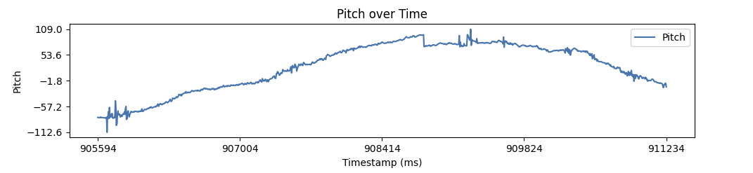
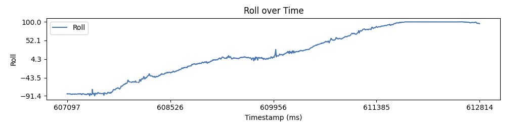
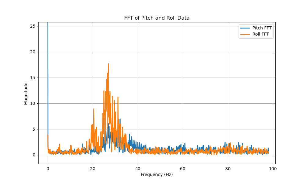
This equation is implemented below in code on lines 16-17.The following figure illustrates the frequency domain signal of the low-pass-filtered pitch and roll. The magnitudes of disturbances are significantly less compared to the unfiltered version.
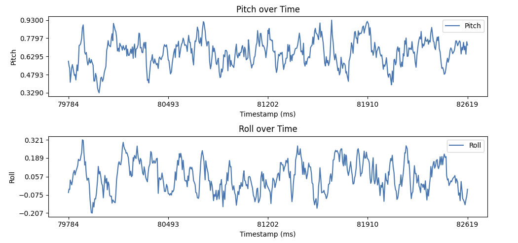
The following figures illustrates the difference between the low-pass filtered pitch and roll and the unfiltered pitch and roll. The low-pass filtered pitch and roll are smoother and have less noise compared to the unfiltered pitch and roll.
Gyroscope
The gyroscope measures angular velocity in degrees per second. We integrate these measurements to
calculate pitch, roll, and yaw. However, because we base new calculations off of past
measurements, errors accumulate. This causes drift in our measurements. The code below runs on
the Artemis board and calculates the pitch value based on gyroscope measurements.
This function is called in the handle_command() function within our bluetooth
interface. This is shown below.
The GET_GYRO_DATA command is sent via BLE from our Jupyter instance get the
gyroscope pitch, roll, and yaw
values from the Artemis board for 1000 samples. A extract_gyro_data(..) function
parses the received strings and processes them into arrays for plotting.
With no delay in our
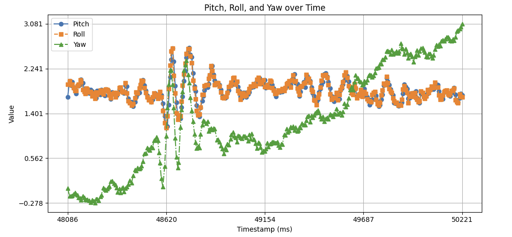
sampling loop, there is some drift. Within 3 seconds, the Yaw value climbed ~4 degrees.
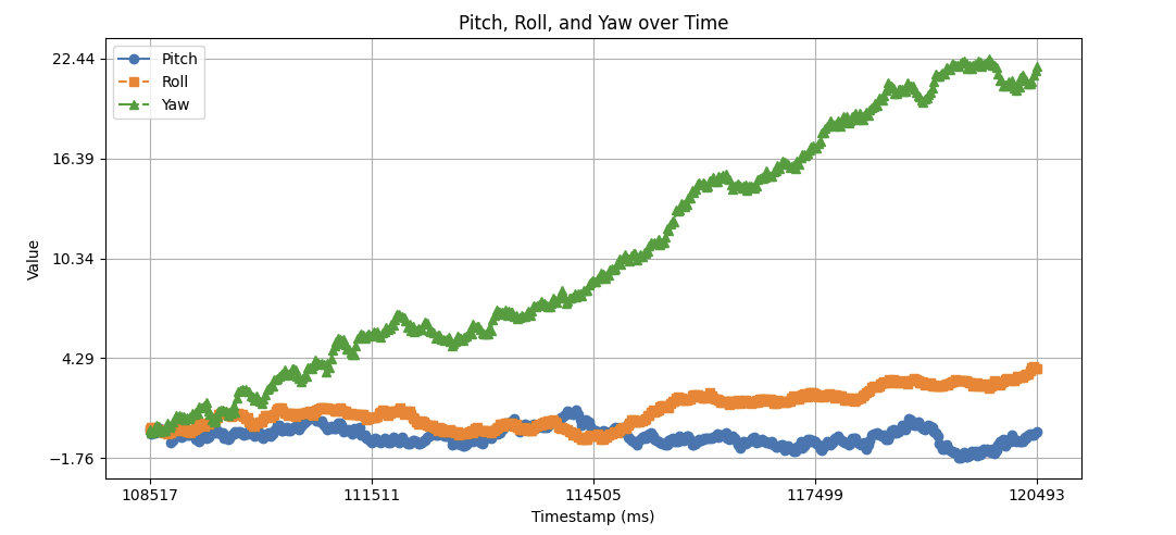
With a 20ms delay in our sampling loop, the drift significantly increased. Within 12 seconds, the Yaw value climbed ~22 degrees. With a delay in our loop, inaccuracies in our gyro measurements are compounded due to the larger timestamp. This results in a larger drift.
To decrease the effect of drift from the gyroscope and noise from the accelerometer, a complementary filter is used to combine the accelerometer and gyroscope data to calculate pitch and roll. The \( \alpha \) value determines the weighting between the accelerometer and gyroscope values. The following equation is used to calculate the pitch and roll.
\[ \theta_{\text{COMP}} = \alpha \cdot \theta_{\text{GYRO}} + (1 - \alpha) \cdot \theta_{\text{ACCEL}} \]
From observations, the accelerometer is a better estimator of our current attitude compared with the gyroscope for most samples larger than a few seconds. With this justification, a \( \alpha \) value of 0.8 is chosen.
The following code is used to calculate the roll using the complementary filter.
The following code is used within the handle_command() function to send our filtered
data to our Jupyter instance.
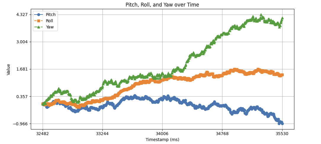
The following figure illustrates the pitch, roll, and yaw data with pitch and roll calculated using the complementary filter. The amount of noise and drift is reduced when compared to the pitch and roll of the accelerometer and gyroscope in isolation respectively.