LAB 7: KALMAN FILTERING
Estimating Drag and Momentum
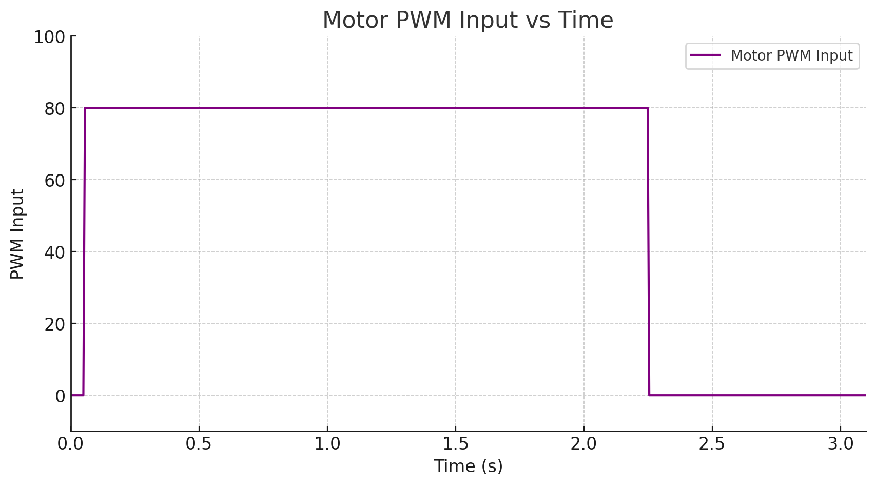
To find the drag and momentum coefficients, data from a step response is logged. To simulate a step response that simulates the dynamics of the PID control in lab 5, a PWM value of 80 is selected to correspond with a u term of 1.
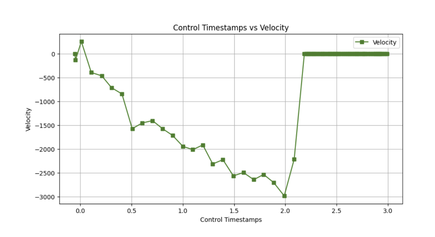
The graphs for TOF sensor output, the car's velocity, and motor input vs time (seconds) are shown below. A linear fit on the section of the TOF sensor output vs time is also shown.
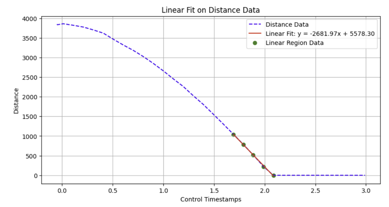
The linear fit region of the TOF sensor output vs time graph is used to calculate the drag coefficient. The linear fit is represented by the equation:
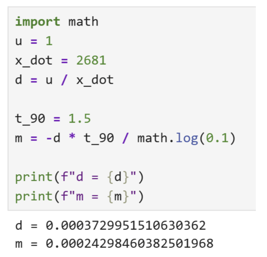
Taking the derivative of the linear fit indicates that the steady state speed is 2681.97 mm/s. The drag coefficient is calculated to be
The momentum term is found using the 90% rise time. From my data, a rise-time of 1.5 seconds is roughly selected. The momentum coefficient is calculated as
Initializing the Kalman Filter (PYTHON)
With our drag and momentum coefficients determined, we can initialize our A and B matrices.
\[ A = \begin{bmatrix} 0 & 1 \\ 0 & -\frac{d}{m} \end{bmatrix} = \begin{bmatrix} 0 & 1 \\ 0 & -1.53505673 \end{bmatrix} \]
\[ B = \begin{bmatrix} 0 \\ \frac{1}{m} \end{bmatrix} = \begin{bmatrix} 0 \\ 4115.4879 \end{bmatrix} \]
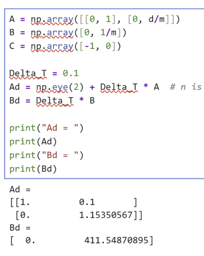
The discretized A and B matricies are initialized as shown below. The Delta T is the time between TOF sensor readings. The time between control loop executions is logged. Taking the mean of these values, we can calculate the average time between control loop executions to be 0.1s.
\[ A_d = I + \Delta T \cdot A = \begin{bmatrix} 1 & 0 \\ 0 & 1 \end{bmatrix} + 0.1 \cdot \begin{bmatrix} 0 & 1 \\ 0 & -\frac{d}{m} \end{bmatrix} = \begin{bmatrix} 1 & 0.1 \\ 0 & 1 + 0.1 \cdot \left(-\frac{d}{m} \right) \end{bmatrix} = \begin{bmatrix} 1 & 0.1 \\ 0 & 1.15350567 \end{bmatrix} \]
\[ B_d = \Delta T \cdot B = 0.1 \cdot \begin{bmatrix} 0 \\ \frac{1}{m} \end{bmatrix} = \begin{bmatrix} 0 \\ \frac{0.1}{m} \end{bmatrix} = \begin{bmatrix} 0 \\ 41.154879 \end{bmatrix} \]
The C matrix represents the states we want to measure. Since we want the measure the car's distance away from the wall, we choose C as [-1, 0].
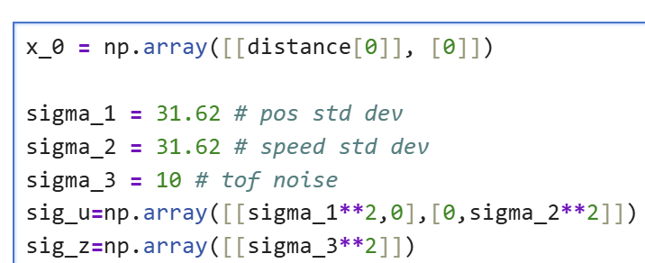
The state vector x is initialized as [[-TOF[0], 0]]. This represents the initial distance from the wall.
The covariance matricies for model and sensor noise are also initialized. For sensor noise, we found the standard deviation of the TOF sensor with a 100ms timing budget to be ~5 mm. This comes from experiments performed in lab 3 that measured standard deviations of different timing budget estimates. As a rough estimate, this standard deviation is set to 10mm to account for EMI from the motor control signals. THe measurement noise covariance matrix looks like this:
\[ \Sigma_z = \begin{bmatrix} 10^2 \end{bmatrix} \]
To calculate the process noise for ouir model's position and velocity, the following equation is used. The 10 term is an estimate of the mm and mm/s difference of the car's position and velocity after one second.
\[ \sigma_{\text{process, velocity}} = \sqrt{10^2 \cdot \frac{1}{0.1}} = \sqrt{100 \cdot 10} = \sqrt{1000} \approx 31.62 \]
Using our estimates for the standard deviation of process, velocity and sensor noise, our model covariance matrix looks like this:
\[ \Sigma_u = \begin{bmatrix} 31.62^2 & 0 \\ 0 & 31.62^2 \end{bmatrix} \]
Implementing the Kalman Filter (PYTHON)
The Kalman Filter is first implemented in Python and fitted to TOF distance data obtained in lab 5. The Kalman Filter is implemented as follows:
With the initial state, model, and sensor noise outlined in the previous section, we can then loop through the TOF data and motor control input data to calculate the Kalman Filter's predicted distance. The sigma matrix is the initial guess of the covariance matrix for the position and velocity uncertainty. The PWM is scaled by the max pwm value to a simulate a u term that is at most 1.
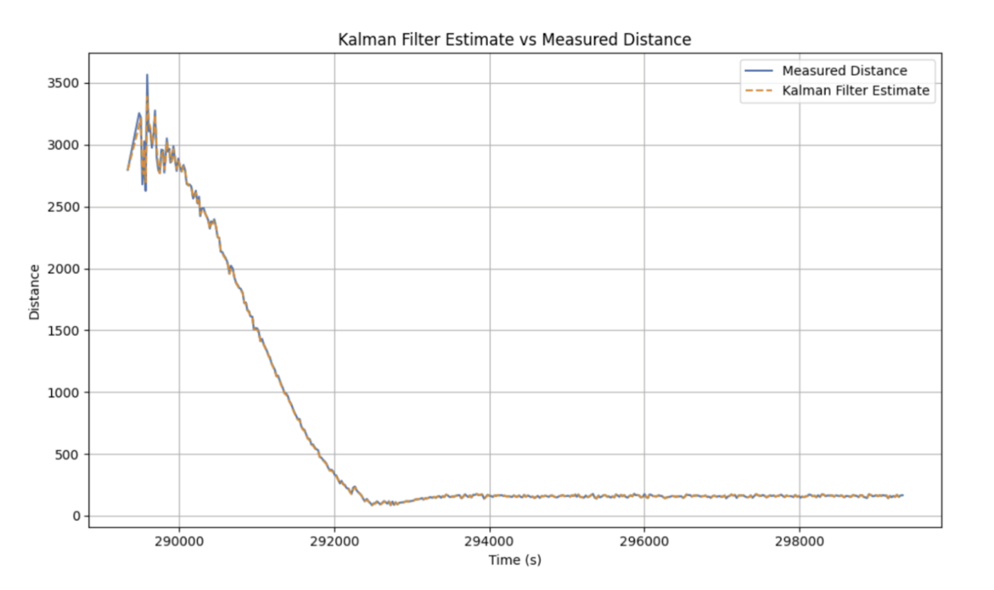
With these initial values, the Kalman Filter's output versus the TOF sensor data is shown below. The filter output heavily follows the TOF sensor data. This is due to the low relative sensor noise standard deviation of 10 and high relative model noise standard deviations of 31.62.
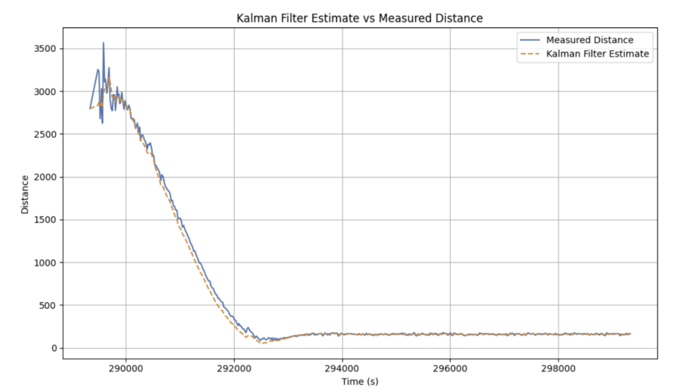
The Kalman Filter is rerun with adjusted sensor and model noise values. The sesnor noise standard deviation is adjusted to 30 while the position and velocity model noise standard devation are changed to 10. This yields the following graph with higher trust in the model and lower trust in the sensor. The estimated distances are smoother and less noisy than the TOF sensor data.
Along with the model and sensor covariance matricies, other factors include the initial state and covariance of our model. Poor initial guesses may lead to poor or high convergence times. Similarly, with a inaccurate initial covariance, the filter may be overconfident in its initial state and be less likely to adjust. The drag and momentum terms also effect performance. If the drag and momentum create accurate state transition and control input matricies, then the dynamics of the system are well-modeled and allow for accurate filter predictions.
Implementing Kalman Filter on the Robot
A function KF(..) is created that takes in a flag that indicates whether data is ready, the scaled control input, and the distance from the TOF sensor. The function updates the Kalman Filter's predicted state and covariance matrix. If we do not have a new data point, no update step is needed.
This function is called inside the PI control function each iteration. The nonBlockReadTOF1(&distance) function indicates whether to set the data ready flag and returns the distance if data is ready. We then pass this flag, the last scaled control input, and the distance read by the TOF sensor to KF(..). The Kalman Filter's prediction and/or update are available in the global matrix x where x(0,0) represents the prediction of the distance from the wall.
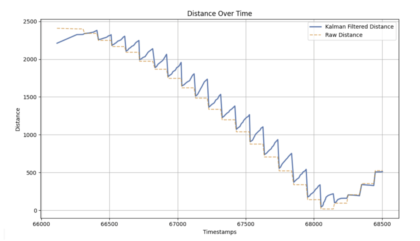
The Kalman Filter's predictions were initially being made in the wrong direction as shown below. When a new TOF sensor reading is made, the Kalman Filter jumps down to the new TOF sensor reading. However, when data is not ready, the Kalman Filter predicts increases in distance, indicating that the car is moving away form the wall. This is fixed by inverting the sign of the control input.
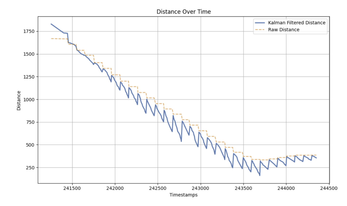
Once predictions are made in the correct direction, the Kalman Filter's output is shown below. The Kalman Filter seems to overpredict the speed of the car.
\[ B_d = \Delta T \cdot B = 0.1 \cdot \begin{bmatrix} 0 \\ \frac{1}{m} \end{bmatrix} = \begin{bmatrix} 0 \\ \frac{0.1}{0.00030778} \end{bmatrix} = \begin{bmatrix} 0 \\ 32.49069 \end{bmatrix} \]
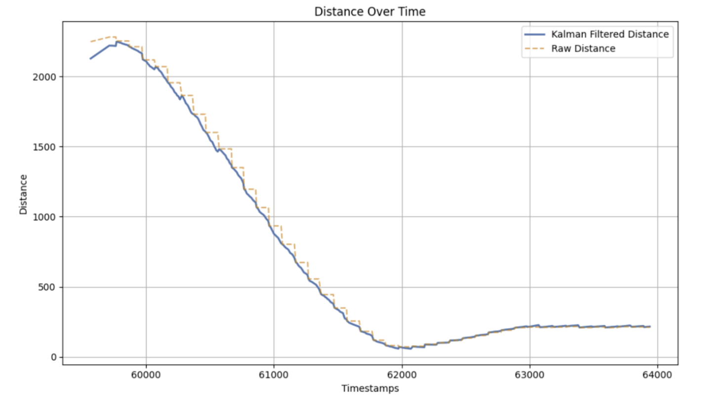
With this change, the Kalman Filter's output and the TOF sensor output is shown below. The Kalman Filter's output is much smoother and aligned with the TOF sensor data. The Kalman Filter's sensor and model noise values were kept consistent.
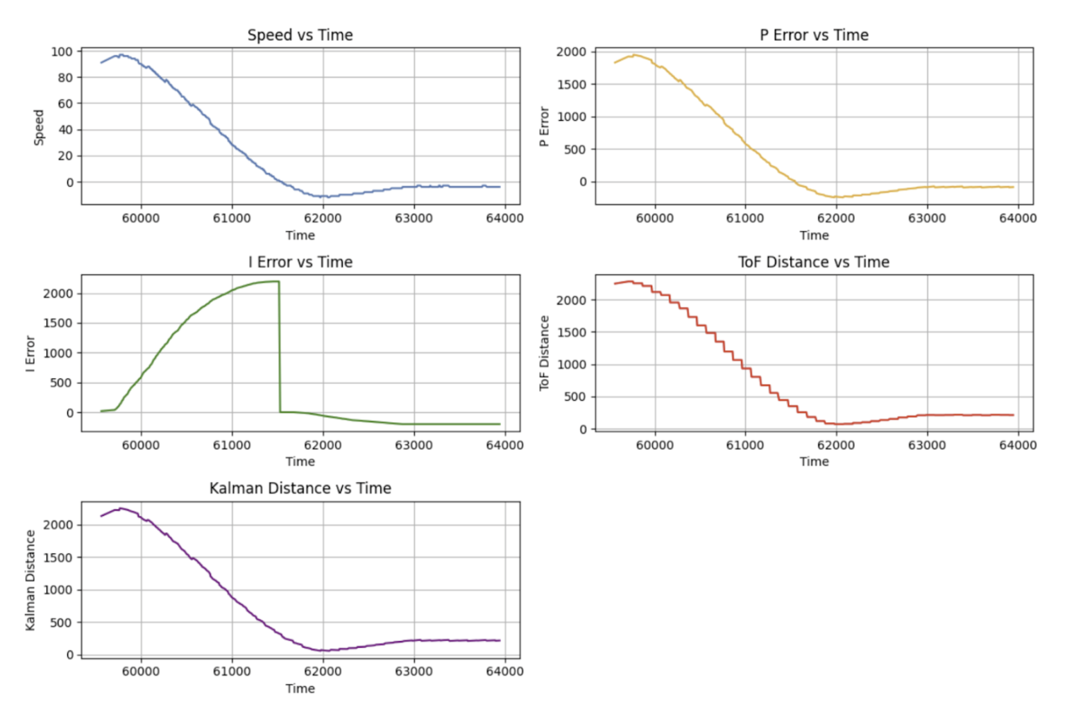
Graphs are shown below of running PI control with the Kalman Filter, a max speed of 110, and a target distance of 300mm. This is a substantial increase from the 80mm max speed with linear interpolation in lab 5. Furthermore, lab 5 was run on carpet with higher friction while this lab was run on a tile floor.